Management Accounting - Decision-relevant Management Accounting

Dynamic Capital Budgeting

Financial evaluation of multi-year projects at the time of decision-making.

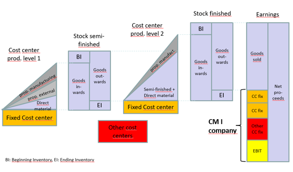
Dynamic Capital Budgeting

The basic principle of an investment: Money is spent today in order to have more cash returns or less cash outflows in the future. Companies, NGO’s, NPO’s and private investors have to decide again and again whether they should invest their available money in companies, plants or process improvements. An investment decision requires a plan-calculation, which should show whether the planned cash outflows and cash inflows can achieve a return in line with the market during the expected useful life of the investment.

Usually investments are expenditures for the provision of a service potential that are intended to generate higher cash inflows or reduced expenditures during the planned period of use.

Simple example 1: Contracting out the maintenance of the garden surrounding the plant to an external organization.

Consequences of this decision are: Additional expenditures for the grounds maintenance contract and eliminated expenditures for paying the former in-house gardener.

Complex example 2: Production and sale of a new product group by an existing company.

In example 1, from a financial point of view it is sufficient to compare the balance of the expected payments for the grounds maintenance contract with the personnel costs for the work previously performed internally.

In example 2, additional net sales and thus additional contribution margins are to be achieved with a newly introduced product group. To generate these additional cash returns initial investments in fixed assets will be necessary, the expansion of net revenue will increase receivables and inventories, and more personnel will be required in individual functional areas. These actions will lead to additional cash outflows. It should also be taken into account that both net revenues and cash outflows will be subject to the life cycle of this new product group, i.e. will lead to different net cash flows in each year of the investment project.

In both cases, cash flow analyses must be prepared for the upcoming decision. For the more complex example of the introduction of a new product group, these considerations must be prepared for a multi-year horizon, because the inflows and outflows of money can occur in different years. In our experience the following structure is suitable for this purpose:

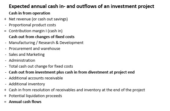
Dynamic Capital Budgeting (only planned values)

This structure can be used generally for investment appraisals, since it contains all elements of cash inflows and outflows. Regarding example 1, the cash outflows would be the payments for the grounds maintenance contract, the cash inflows would be the saved cash-out personnel costs for the previous employee. The introduction of a new product group (example 2) requires the entry of all items listed in the table above because this investment project affects both the income statement and the balance sheet.

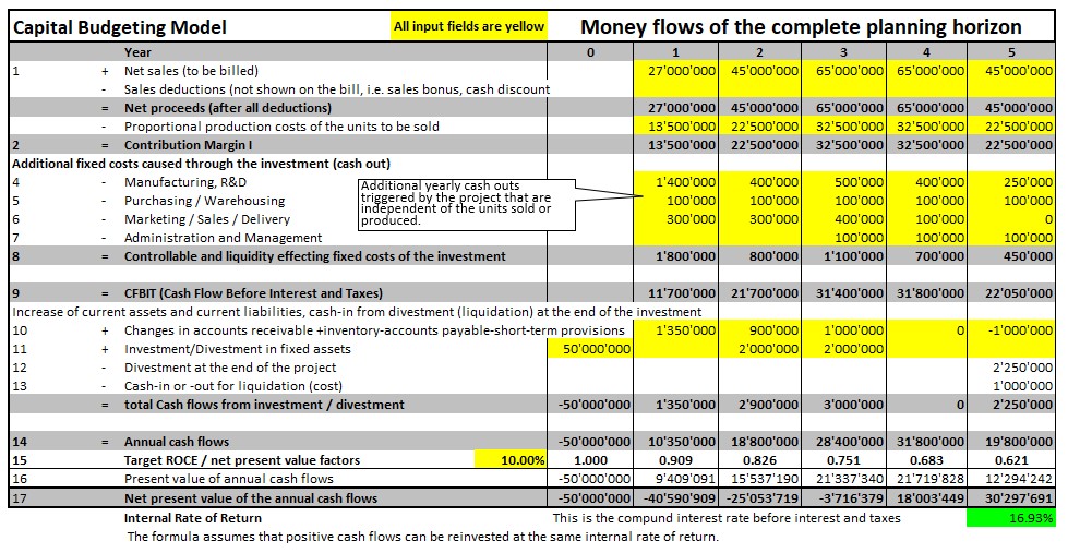
Therefore, it is advisable to prepare the investment appraisal in such a way that the expected annual cash flows can be identified and discounted for each year. In the product launch example, these cash flows are planned as follows:

Capital Budgeting Model — Present Value of an Investment

- Year 0 is the beginning of the implementation of the decision. The main investment of 50 million has to be paid then (line 11). For the years 2 and 3 it is assumed that additional investments will be necessary to increase the production capacity of the plant.
- The annual net revenues expected from the project are entered in line 1. The development of the net revenue corresponds to the expected life cycle of the new product.
- In line 2, the planned proportional costs of the expected yearly sales are calculated (50%).
- In year 1, further payments of 1.0 million are incurred for introductory work. In addition, it is expected that the staff in Production Planning and Control will need to be increased, resulting in 0.4 million additional annual expenditure (line 4).
- Further additional personnel are required in the areas of purchasing and warehousing as well as marketing / sales / distribution. The expansion of the business volume will also require an additional person in administration in the years 3-5 (lines 5-7).
- The total annual cash outs for internal tasks of this project (additional personnel) can be seen in line 8).
- Line 9 shows the net benefit of the investment project (yearly net cash inflows).
- Lines 10 and 11 show the net impact of the project on fixed assets, accounts receivable and current liabilities over the years.
- At the end of the project (here year 5), the built-up receivables and inventories are liquidated again. There may also be liquidation proceeds for the asset that is no longer in use (lines 10, 12 and 13).
- The annual balance of cash flows is shown in line 14.
- The example shows 5 plan years but can be extended for more years as needed.

Adding up the nominal yearly net cash flows in line 14, it can be seen that the investments will be completely paid back during year 3 (simple payback period).

The time value of money

Anyone who provides money, whether it is the company itself or an investor, expects to be remunerated for this service in the form of interest. If, for example, an annual interest rate of 10% corresponds to current money market conditions, a company must pay an interest of 100 for a loan of 1,000 at the end of a year. If the lender is to make the money available for several years (example 2), he will ask himself whether he will be remunerated for his investment with compound interest. Consequently, from his point of view he wants to know at the time of decision what the present value of the investment will be over the entire term of the loan and whether this return will stand up in comparison to other possible investments.

Investors therefore ask themselves: How much will I get back for my investment at the end of one year or at the end of the project? If, as in the example, he sets a target interest rate of 10% per annum, the result is:

Interest for 1,000 investment amount = 10% * 1,000 = 100 p.a.

The 100 are to be paid at the end of the year. So the value of the interest payment at the beginning of the year, respectively at the time of the decision for the investment is 90.9091 ((100 : (1+interest rate 10%) = 90.91).

If the interest of 100 accrues only at the end of year 2, the 90.91 must be divided again by the interest rate (90.91 / (1+interest rate)) = 0.826). In the compound interest calculation, the formula 1 / interest rate ^number of years is used. This results in the present value factors, which are shown in line 15 for the rate of 10%. The corresponding present values of the plan years are shown in line 16. Line 17 shows that the accumulated present values will only at the beginning of year 4 be sufficient to pay for all the investments and divestments and for the 10% compound interest (lines 10 and 11) at 10%.

Overall, according to the plan, by the end of year 5, the cumulative present values in example 2 should be 30.298 million higher than the net investments in all the years of the project. In setting up the example, it was assumed that the life cycle curve of the product group will go through its build-up and growth phase in years 1-2, will reach saturation in years 3 and 4 and that the phasing-out of the life-cycle will begin in year 5.

Pitfalls in the application of Dynamic Capital Budgeting

- Depreciation has no place in an investment calculation. This is because by taking the investment amounts into account the cash outflows are already included.
- Likewise, tax consequences of investments are generally not included, since the profitability rate to be achieved refers to the profit before deduction of interest and taxes.
- Saveable tax amounts are also not relevant to the decision because taxes are calculated from the reported profit after interest. The latter can also develop negatively if an investment project is going well but the market situation leads to a drop in sales of other products and thus to less annual profit.
- As the name implies, capital budgeting is a forward-looking view. The method is always based on planned quantities and values because it is intended to support decision-making in strategic and operational planning. Whether the investment has really increased productivity can only be determined by evaluating the actual data from management accounting.

With the present-value approach the investment appraisal becomes dynamic.

Download the Excel model for the quantification of investment projects here and adapt it to your own needs. Copying the formulas in new rows allows to include additional years. The model is particularly suitable for the quantification of strategies. With the help of the Excel formula “Internal rate of return” also the internal rate of return of the project can be calculated (see the 16.9% on the right in line 18). This helps to compare competing projects. But it should be noted that this formula assumes that cash returns can also be reinvested at the rate of 16.9%.

Market rate of interest

In the presented example an interest rate of 10% was assumed. But which interest rate should be applied for the assessment of a real project plan or a general investment?

For this purpose, the interest rate in line with the market for companies with the same risk must be determined. The procedure for doing this is described in the post “Profit in Line with the Market“. There, it is also noted that the 10% assumed in the example above correspond to the market reality in German speaking countries and in the US.

Dictionary of Management Control and Controlling

Because many organizations operate internationally, communication is increasingly multilingual. For this reason, we have expanded and updated our overview of technical terms in the world of controlling and management control systems.

Find more than 2,500 technical terms in English, German, French and Italian.

Click here to download your copy of the Excel-file.

It will appear in your download area from where you can save and complement it with your own technical terms.

Activity Based Pricing

It seems more interesting to use the activity-based idea for finding, setting and negotiating sales prices, that means, for Activity Based Pricing than for costing.

Activity Based Pricing

Five of ten case studies published so far by the Profitability Analytics Center of Excellence PACE (see Management Accounting Practice Reports) deal with the question of how the unequal, only partially measurable use of a company’s support areas and capacities can be taken into account in sales pricing for different customers.

Specifically, the following cost pools should be included in sales pricing for different customer/product combinations:

- Costs of procurement and warehouse logistics, which vary for different product groups,
- Scrapping costs for expired or unsaleable products per product group,
- Distribution costs such as transportation, storage, replenishment of shelves, delivery cycle (daily, weekly, monthly) per customer,
- Customer care costs for order processing, handling of returns and complaints and general support by the sales force.

Although these fixed cost blocks cannot be allocated to an individual product according to cause, it is possible to calculate average values per activity and then take these into account when setting prices for different customer groups or sales channels.

This does not change anything in the management accounting system or in the contribution margin methodology, nor does it change the decision-relevant internal inventory valuation (at proportional standard costs). This is because fixed cost center costs are related to executed processes.

Activity Based Pricing is intended to support marketing- and salespersons in justifying the estimated costs of fixed cost processes to customers. For this purpose, it is not necessary to adapt the management accounting system, which is used for planning and control, but parallel calculations can be created.

Application example Ringbook Ltd.

For the example company Ringbook Ltd. the following table shows the fixed costs for 2021 at the lowest product level to which they can still be clearly allocated, i.e., without using any fixed cost allocation factors.

Of the total fixed costs of around 3.48 million, 1.44 million can be allocated to the two product ranges, while 2.04 million are incurred for the entire sales organization. The fixed costs for purchasing and warehousing were broken down in proportion to the purchasing values of the areas (own products, merchandise, investments and projects (general)). This took place under the arbitrary assumption that the costs of the purchase department are driven by the purchase volume.

With this classification the lowest level of the allocation of fixed cost blocks is reached in the example company. For:

- Sales promotion is performed in each case for all products of a product range, for all customer groups together.
- In sales and marketing all products are sold to all customers and a sales order can include one or more positions.
- In production, manufacturing orders are processed for both semi-finished and finished products, which is why their fixed costs are incurred for all manufactured goods.
- Administration and management work for all products.

The next part of the table (lines 7 – 14) is based on the proportional manufacturing costs of the products sold in the two assortments of own products and merchandise. Since the calculation is based on bills of materials and routings of the individual articles and the purchase prices for the individual merchandise products are known, their proportional costs can be calculated for each assortment according to their origin (line 7). From this, the proportions of the general fixed costs per assortment can be calculated in lines 8 and 9 (89.4% and 10.6%). In line 10, the directly attributable fixed costs are taken from line 6 of the previous table. This results in the full costs per product range in line 11.

Activity based picing — Activity Based Pricing

Comparing the net revenues in line 12 with the calculated full costs in line 11, reveals the calculated EBIT per product range (line 13). The total EBIT of 294,347 corresponds to the EBIT in the P&L (line 14).

After this allocation of fixed cost blocks to products it can be seen that the large share of EBIT comes from the own products. This was already apparent from the stepwise CM-calculation.

If the activity-based fixed cost allocation presented here is taken as the basis for pricing, the prices of merchandise would have to be increased and those of the own products reduced. In this way, the merchandise would achieve a higher calculated EBIT and the lower prices of the own products would allow sales volumes to be increased. However, the merchandise range has only been sold for two years, so it is still being built up. The sales prices have been set by observing competitor prices, so a price increase would lead to a drop in sales. Otherwise it makes no sense to lower the prices of own products, because no significant increases in production volumes are possible with the existing production capacities.

In summary, for the estimation of activity costs the fixed costs of a cost center are to be assumed and these are to be compared with the process quantities. Using the example of a purchasing department it is understandable that an initial purchase from a supplier takes more time than a reorder. The personnel costs in the marketing department for producing a sales catalogue remain the same whether one or thousands of catalogues are printed. But the full cost of one catalogue will change. The question whether the costs of the catalogues are to be split between existing and potential customers remains open.

Outlook

The more interwoven the internal service relationships are in the production and marketing of products, the less meaningful a cost-based sales price calculation becomes.

For the determination of gross and net sales prices, the allocation of fixed costs to customers and products can be a support. However, the net prices of competitors are more important.

Activity Based Pricing should in any case take place outside of Management Accounting. It is used to set prices but does not directly change any costs.

Complete Variance Analysis

Planned to actual comparison in stepwise Contribution Margin Accounting shows where corrective measures must be taken first.

Complete Variance Analysis

The step-by-step contribution margin accounting, also called sales performance accounting, allows for a complete variance analysis. All variances from plan are to be identified and analyzed to derive corrective measures or new plans.

In the report for year 20XX of Ringbook Ltd. it can be seen that

- Gross sales grew mainly due to increased sales in the merchandise product range (+36.9%). In both assortments, somewhat higher sales deductions were granted in order to realize the sales. As a result, CMI I as a % of net sales for merchandise fell by 3.36%. Overall, the absolute CM I increased by 105,810 (see yellow fields).
- Sales promotion costs (fixed costs of the product groups) are clearly attributable to assortments but not to individual product groups. They did not deviate significantly from plan. The cost centers sales management and sales territories show minor spending variances in their cost centers. Since the sales organization works for all products, its fixed costs can only be allocated to the company as a whole (see grey fields).
- The purchase price variances (line 2, red fields) could be assigned to the two assortments because all raw materials and supplies are consumed for the company’s own products. The price changes of the suppliers of the merchandising goods appear in the corresponding assortment.
- Production order related variances can be collected for each production order. Here, the summarized values per variance type are presented for the responsible production management. These variances refer only to semi-finished and finished products manufactured in-house. Therefore, they are shown in the column for the goods manufactured by the company (light blue fields).
- The spending variances (target costs – actual costs) remain. These arise in each cost center per cost-type. In the stepwise contribution margin accounting, they are shown by cost center or summarized by functional area (dark blue fields for production and light green for other cost centers). Favorable spending variances increase the EBIT. They are the expression of the fact that fewer actual costs were incurred than target costs during the period under review. This corresponds to a productivity gain relative to plan.

This company-specific design of the step-by-step contribution margin accounting shows which individual areas of responsibility contributed to what extent to the improvement in EBIT of 93,316.

Purchase Price Variances are topical again

Show purchase price variances in financial accounting per period and in management accounting per product.

As a result of the Corona pandemic and supply chain challenges, increasing inflation rates can be observed worldwide. As a result, the questions of how quickly and comprehensively rising costs can be passed on to customers and what consequences can be expected for the company’s own results are coming to the fore.

To determine the extent to which price variances in purchasing could be passed on to customers and whether price increases are leading to increased spending variances in the cost centers, it is necessary to record purchase price variances in management accounting for short-term planning and control.

In the example below, the real price development for the purchase and consumption of sectional steel is the starting point for determining the company’s own material acquisition costs. Data origin: cf. https://www.d-a.ch/da/da-home/services/dienstleistungen/preisentwicklungen/stahl-metalle/kbob/kbob-preisindizes-baugewerbe.pdf) .

Purchaseprices sectional steel — Purchase prices sectional steel

Row 7 of the table shows the monthly purchase price variances based on the standard price of EUR 120.- per ton.

- These variances should be recorded as part of the monthly cost of materials in financial accounting, since the purchase price variance arose in this period.
- In management accounting, however, the planned standard purchase price should be used throughout the whole year, since otherwise production would have to create a new standard cost calculation every month, which would be too late for sales, since new price increases have already occurred in the meantime.
- The purchasing manager should include the expected average inflation when setting the standard purchase price for the plan year. Since he is not a prophet, he can only estimate the price. This estimate goes into the planned product costing and consequently is also applied in the planned contribution margin calculation. The advantage of this is that the standard cost estimate remains the yardstick and the monthly variances can be calculated automatically.
- Stock receipts of semi-finished and finished products are also consistently valued in Management Accounting at proportional standard manufacturing costs, which in turn facilitates the preparation of contribution margin accounting.

This approach also makes sense because raw materials from deliveries with different real purchase prices can be consumed in the same production order. The table highlights consumption and costs:

- Order 1 (row 8) consumes in January the 100 tons of sectional steel purchased in December of the previous year at a price of 100.00/ton, plus 20 tons from the January delivery at a price of 117.30 (row 3 in the price development table).
- Due to its volume of 320 tons the production of order 4 (row 11) has to be distributed over the months March to May. Because 100 tons are purchased each month and charged by the supplier at the applicable price, 3 different purchase prices would also have to be used for the calculation.
- If the smaller order 5 (row 12) were processed before order 4 in early March, it could still benefit from the more favorable purchase price in February of 134.20 per ton at the expense of order 4, but this would increase the cost of order 4.

This complexity of evaluating order-specific consumption cannot be expected of neither the production managers nor the salespeople. In addition, as can be seen from rows 16 – 18, the valuation rule to be applied would still have to be determined:

1. All purchases are valued at the standard purchase price throughout the year (row 16).
2. The real withdrawals from the warehouse are valued at the current purchase price of the month of purchase (Last-In-First-Out, row 17).
3. The real purchases are valued at the weighted average purchase price of the current inventory (weighted average purchase price, row 18).

It can be seen that price variances in purchasing are period costs. They can only be clearly allocated to a product if the material was purchased directly for a specific production order.

As a result, especially in inflationary times, order and product costing should be carried out using standard purchase prices. Otherwise, those responsible for production will lose their orientation with the use of rapidly changing prices. In addition, they are held responsible for variances for which they are not responsible.

As mentioned, purchase price variances are period costs. In stepwise contribution accounting they can usually not be clearly assigned to a specific sale. Consequently, they are to be reported where unambiguity is given, e.g. per product or customer group or, as in the example, the assortments (cf. Management Control with Integrated Planning, p. 231).

Management Tasks and Management Accounting

Corner stones for the implementation of the decision-relevant Management Accounting System covering revenue, activities, capacities, cost and earnings.

Management Tasks and Management Accounting

The design of the management accounting system outlined in this blog and in the book “Management Control with Integrated Planning” is based on generally accepted management principles and the resulting behaviors.

Decision support and responsibility for results

All managers make decisions and are responsible for their implementation. This applies to all individuals who manage an area and are accountable for its results to their superiors or to the company. Managers of all levels are thus the main customers of the management accounting system. Consequently, such systems must be structured to provide decision support to all managers at all management levels and to delineate responsibilities in a manner that is appropriate to the organization.

To fulfill its purpose, results must be achieved by a company. Objectives are results to be achieved. Each manager should be able to plan, measure and control the achievement of his objectives in accordance with his responsibilities.

As far as monetary targets are concerned, they are to be described in the management accounting system. From this it can be deduced that planning in management accounting should run in parallel with the process of agreeing on objectives. If, for example, the activity quantity of a cost center is determined as a target, but the headcount required for this objective is not approved, it cannot be achieved.

Objectives and plans belong together

When planning, it is necessary to make and prepare the decisions regarding personnel, material and financial resources required to meet the strategic and the operational goals. Since this process is time-consuming, ways are often sought to simplify and shorten the planning process. Despite the large amount of work involved, however, practice shows that it is worthwhile to plan all areas, products and management levels once a year in terms of performance and value and in conjunction with the objectives of an area. This provides the benchmark for the plan to target and plan to actual comparison and thus the basis for determining corrective actions. Planning for a fiscal year also proves useful in “short-lived” times, because personnel and management decisions as well as objectives are usually also agreed for a fiscal year.

The management cycle requires plan, target and actual data

In order for the management cycle to work properly the plans that are created together with the objectives must be stored in the system in all their detail, so that they can be compared with the results achieved. The comparison of planned, target and actual data makes it possible to also measure the actual extent of achievement of the objectives in monetary values. It is recommended to prepare the plan to actual comparison on a monthly basis, so that the real events are still present for the evaluation of the results. It also enables faster reaction in the case of unfavorable variances. For projects, the plan to actual comparison should also be set up for each milestone, because at each milestone meeting a decision has to be made as to whether the project should be continued or terminated (a go/no-go decision).

Managers at all levels usually decide on quantities, activities and times. The value consequences of implementation then become known in cost accounting. This requires that the management accounting system be designed as a cost-, activity-, revenue- and earnings system (CARE). Management-oriented CARE is therefore clearly distinguished from purely money-based financial accounting.

Requirements from strategic and medium-term planning

Strategic planning defines the intended positioning in the markets. For this purpose, product/market positions to be achieved are specified with quantities and revenues for several years.

Medium-term operational planning has the task of preparing the implementation of the strategies. Since the managers must record quantities, services and prices for this purpose, the CARE structures must also be set up in the multi-year planning.

In annual planning, the planned purchase prices, the planned personnel costs, and the bills of materials as well as the work plans for the planned year are set. This results in new planned cost center rates and new planned product costs.

Adjustments at the beginning of the new year

To enable managers to compare their achieved results with the planned values at any time during the year, the inventories of materials, semi-finished and finished products in CARE must be revalued using the new approach at the beginning of the next year.

If, for example, a product can be manufactured at a lower cost in the new year due to a process improvement, the previous year’s ending inventory must be revalued internally with the new cost rates. If this revaluation of the year-end inventory is not carried out, variances will occur in the new year which still belong to the old year. This revaluation is only carried out in management accounting and can be automated. Inventory valuation for financial accounting continues to follow the applicable commercial law regulations.

Forecasts

Because the preparation of forecasts ties up a lot of management capacity, it is advisable to schedule two forecast dates. When the fiscal year corresponds to the annual calendar, the first forecast should be prepared on the basis of the planned and actual data from January to April (Easter days are then always included). Based on the accumulated actual values as of the end of August (major vacation period mostly completed), the second forecast should be prepared. This forecast also serves as the input for the subsequent planning of the next business year. Stock-listed companies are usually forced to prepare quarterly forecasts. However, practice shows that especially forecasts based on the actual data as of the end of March is not very meaningful, and its preparation usually causes a lot of hectic activity in the organizations.

Controllers check the right system application

As designers and operators of the management accounting system, controllers have the task of monitoring the correct application of the planning and controlling system. This results from the controller mission statement (see Management, Controlling, Controller). Once the planning results or forecast data have been entered into the management accounting system, a sufficient period of time must be provided during which the controllers can check compliance with the system rules and, if necessary, ensure that corrections are made on time. Unfortunately, there are always “specialists” who try to abuse the planning system or valuation rules in their favor by circumventing content-related or process-related rules:

- In a company known to us, a business unit manager massively manipulated the planned net attendance times of the employees in order to be able to calculate lower unit costs in the plant he wanted to erect. On this basis, the investment in the plant was approved by the group’s management. In the first year of operation it already became apparent that the actual attendance times did not correspond to the planned ones, which led to the loss of the planned cost savings. In retrospect, the desision to make the investment had to be judged as wrong, but the money had already been spent.
- In multinational companies, there is a great risk that decisions about the profitability of a subsidiary are made on the basis of transfer prices between group companies. However, the latter are driven by international transfer pricing regulations obeying legal requirements and leaving out the overall group view (each country wants to generate taxes locally for the value produced, making it difficult to properly charge group services back to the producing and selling individual companies).
- From a controllers’ view, planning for an individual company must therefore be based on local conditions, but must also take into account the group’s internal planning and control requirements (those parameters which the local managers can actually influence themselves and therefore also take responsibility for). From this it can be deduced that controllers must set up the management accounting system in such a way that the entire business can successfully be managed locally. The finance department at corporate headquarters, on the other hand, must use transfer pricing to ensure that the overall corporate tax burden remains as low as possible (tax optimization). From a management perspective, these two areas must be kept separate if local planning and management are to be carried out correctly and the group result optimized.

Design of the decision-relevant Management Accounting System

To design a comprehensive management accounting system that can meet the requirements resulting from the management process, we have been observing the scientific developments as well as their practical implementations at our customers for several decades. According to our findings, the following sources and systems are of decisive importance for the design of CARE:

- Marginal costing according to Hans-Georg Plaut (Grenzplankostenrechnung GPK)
- Standard costing with flexible budgets according to Wolfgang Kilger
- Contribution margin accounting according to Albrecht Deyhle
- Sales and turnover planning according to the lived market cultivation structures
- Extension to multi-level and multi-dimensional contribution margin accounting (mainly described by Lukas Rieder)
- Three dimensions for the management-oriented structuring of costs and revenues in the controller dictionary of the International Group of Controlling (IGC)
- Activity Based Costing (ABC) according to Robert Kaplan and Peter Norton, but without allocation of fixed costs (including capacity costs) to product units. This mainly corresponds to Resource Consumption Accounting (RCA)
- The Costing Levels Continuum Maturity Model by Gary Cokins
- The IMA (Institute of Management Accountants) Conceptual Framework for Managerial Costing.

References to these publications can be found in the bibliography of this blog.

Multidimensional Contribution Accounting

A truly helpful management accounting system must deliver its figures in plan and actual according to market dimensions and internal structures. Only then it enables correct decision-making. Multidimensional and multi-level contribution accounting is the instrument for this.

In accordance with the goal orientation in the entire management (see the post “Integrated Management System”) it is also necessary to record values to be achieved for specific persons in the income statement. Multidimensional contribution accounting can make a significant contribution to this.

Multidimensional contribution accounting

Contribution accounting must be structured according to the structures in the company. For the example enterprise, the following plan results: We start with the sales and the sales deductions. The proportional standard product costs are deducted from these, which results in the Plan CM I. The planned sales commissions are subtracted from this. This in turn results in Plan-CM I after sales commission of 3,668,723.

The two assortments and the product group structure are shown horizontally. In this way, the CM I for each product group is visible. In the simulation model, this observation is possible at the individual item level.

This means that all proportional costs of sales are included (withdrawal from the finished goods warehouse at standard). Vertically, the fixed cost center costs are assigned to those areas where they can be clearly influenced and thus justified. The entire process of showing directly controllable fixed cost blocks is based on this responsibility without using any keys for fixed cost allocation:

- The company plans the costs for sales promotion in the cost centers “Sales Promotion Own Products” and “Merchandise”. These are fixed product range costs that can be assigned uniquely to the assortment, but not to the product groups or even the individual articles.
- The sales area consists of the three cost centers for the sales areas and those for sales management and internal sales. As these organizational units sell all articles of Ringbook Ltd., the fixed sales costs can only be assigned to the total of all contribution margins.
- The total fixed costs of the production area (995,112) can only be clearly assigned to the range of own products, since the employees take care of all own products.
- The remaining cost centers from the warehouse to management and administration work for the entire company, which is why they are only presented in the “Total company” column.

The result is the planned EBIT (earnings before interest and taxes). Assuming that the EBIT of 201,058 also corresponds to the profit objective for the year, the following responsibilities can be derived:

- The company manager is responsible for achieving the planned EBIT.
- The cost center managers are responsible for keeping to their target costs. These are the planned costs of the activity actually performed (explained in detail later). In all cost centers that are not directly involved in product creation (that is, they do not appear in any work plan), the target costs correspond to the planned fixed costs.
- The head of procurement is responsible for realizing the planned (standard) purchase prices.
- The top sales manager is responsible for the complete sales-CM. This includes the net revenues, sales commissions, planned proportional cost of goods manufactured, and the fixed costs of the entire sales organization. This responsibility can be partially delegated to sales area managers, since they are responsible for the CM achieved in their area and their own fixed costs. It can also be delegated to assortment managers or heads of promotion areas. If there is responsibility for both, regions and assortments, this results in a “crossed responsibility” (more to this at the end of this post).

These explanations are intended to show that the structure of the multilevel contribution accounting system allows obtaining financial targets that fully correspond to the ideas of Management by Objectives. It is important that the multilevel CM-calculation is designed according to the conditions and structures of the company (not according to the textbook).

If the sales, turnover and net proceeds are planned in all relevant dimensions of sales as described in the post “Planning from the Market into the Company”, the CM calculation can be created not only multilevel but also multidimensional. The prerequisite is that both product and customer structures are structured and planned bottom-up.

Contribution margin accounting for the sales areas is created by evaluating sales planning according to sales areas and the cost centers assigned to them. Each area manager has his own cost center for which he plans the fixed costs, which he can directly influence and therefore be responsible for. These are fixed costs because they have nothing to do with product manufacturing, but with the sale of all items. If this cost block is subtracted from CM I after commissions, the area CM (sales region) is the objective to be achieved.

Planned contribution margin for sales regions and sales management

No fixed costs were directly assigned to exports because the sales manager together with his office staff wins and handles all foreign sales in addition to his management task. According to this organization, the fixed costs of exportations are included in the cost center sales management and internal sales support. Using an appropriate allocation basis, these fixed costs could be distributed between export and sales management. But the consequence would be that nobody would be responsible for the fixed costs of internal services neither for exportation. This example shows why the structure of the database and of the profitability analysis always has to be set up according to the organizational circumstances.

The sales contribution of 2,495,958 is the same as the one in in the dimension of product groups. All the fixed costs below remain the same since the cost centers for production and the other areas work for all sales areas. This again results in the same EBIT.

The salespersons planned sales volumes and revenues per product group and sales area, but not by sales channel. Therefore, in planning, CM-accounting cannot be created according to sales channels. In the actual view, however, this will be possible, since the customer number in the invoices indicates the channel to which the customer belongs.

Today it is common practice in many companies to cultivate the market along various dimensions (for example, territories, sales channels, product groups). For each of the dimensions, the same total sales and contribution margin totals are to be achieved. As mentioned, the top sales manager is responsible for the complete sales CM. In order to achieve it area managers must coordinate with product managers. A sales promotion campaign for certain products (or product groups) should result in salespersons specifically recommending the respective products in their presentations and making targeted use of any available advertising material.

This coordinated approach can be supported by cross-referencing the results targets. The columns show the contribution margins planned in the individual sales areas for each product group. In the rows, the sales promotions planned for the product groups are compared with the target CM. It can be seen that the budget for the promotion of the still small merchandise area is almost as large as that for the own products. The intention here is to promote the merchandise area. This requires salespeople making their customers more aware of the advantages of the merchandise assortment.

Contribution accounting in two market dimensions

Contribution margin accounting is a powerful tool to support objective-oriented approaches and, in particular, for promoting coordination between all areas of an organization. It can be adapted to changing corporate structures. This also applies to strategic planning. Because there it has to be decided with which products the company wants to reach which market positions in the future and thereby make the profit targets become reality. To do this, it is necessary to know which sales volumes and net revenues will be added and which will be eliminated, which costs will be incurred by the products (proportional) and which capacities and structures will have to be rebuilt for the necessary success potential (fixed).

In operational terms, contribution margin accounting helps to enable management by achieving agreement on objectives. It provides the tools for agreeing on targets for sales and net revenues down to the individual order or customer. Cost targets are mapped in such a way that they correspond to the direct influence of the holders of the objectives. The proportional manufacturing costs of an item are the target value for consumption in production. Finally, the planned fixed costs are the budgets for maintaining performance, whether in one area or in the entire company.

Contribution Margin or Full Cost

Full cost accounting leads managers to take wrong decisions because fixed costs are allocated to the costs per unit. Here is the proof.

Contribution Margin or Full Cost? What is decision-relevant?

Thanks to good negotiating of the CEO of Pekka Heating Systems Ltd., his company was able to acquire and realize a large installation order for a university building and a smaller conversion order for the heating system in a house with 6 apartments in the last period. Now the question is what kind of orders should be increasingly won in the future. A consultant was commissioned to calculate whether it would be more likely to win conversion orders or large installations of new systems. The consultant explained that, using the method he knew from school, he had first distributed the full manufacturing costs over the orders according to the number of hours worked. The costs of sales and administration were then allocated to the orders in proportion to the full manufacturing costs.

He presented the following calculation:

Contribution Margin or Full Cost — Full cost accounting

The verdict is clear: it is not advisable to accept large orders.

The project manager of the large installation project was, on the one hand, proud that Pekka Heating Systems Ltd. was able to successfully implement this large order and, on the other hand, frustrated by the massive loss of the order. Therefore he asked a friend if the consultants’ calculation was correct. The friend presented the following table:

Without order 1 the company would be bankrupt

With the following example, the friend showed him that the application of different cost allocation bases (allocation keys) leads to different order results every time, despite the same initial situation. None of the results can be correct because costs are distributed that are incurred for the whole organization.

Different fixed cost allocation keys lead to different order profits

The conclusion remains that full cost accounting is not suitable for management control, because managers need to compare both in planning and in the concrete case of application the additional net proceeds of an additional order to the direct costs incurred with this order.

Precisely because various accounting standards and tax laws require the preparation of full cost accounting, management accounting requires the courage to not allocate fixed costs from one to other cost centers, orders, and products because otherwise managers will make wrong decisions.

Contribution Margins to Cover Structure Costs

Contribution margin accounting is applicable in all industries. The procedure is described using various examples. In addition, the path from the contribution margin of a single item to the EBIT of the company is shown.

After completing the planning for proportional product costs and net revenues (see the post From Planned Sales to Net Revenue), the data to calculate the contribution margins to cover structure costs is available.

Contribution Margins to Cover Structure Costs

The proportional cost of goods manufactured includes those planned costs that are directly caused by the product (valued bills of material and work plans). All product costs are first booked as entries in the warehouse (semi-finished or finished products) at planned proportional costs (standard costs) and are withdrawn from there at the moment of delivery to the customer. The planned fixed costs remain in the cost centers.

The example of item 101060 shows how contribution margin I is created in the plan:

CMI 101060 — Contribution margin of article/item 101060

Salespeople should not get a commission based on sales or net revenue as a component of their income. Doing so often leads to rebates of all kinds being granted in order to achieve the sales targets or to increase capacity utilization. Therefore, in the example company a contribution-based commission of 2% of the achieved CM I volume is credited.

The contribution margin I (CM I) is internationally defined as the difference between net revenue and proportional product costs (see Glossary). It is easy to see that the sum of all CM I must be sufficient to cover all fixed costs and earnings before interest and taxes (EBIT) if the result is to be in line with the objective. CM I is thus the contribution to structural cost coverage. The following illustration shows its creation:

Contribution Margins to Cover Structure Costs — The interaction between production levels, warehouse positions and Contribution margins

The following planned EBIT can be shown in the example company:

This illustration is not particularly informative. In the post “Multi-Level and Multi-Dimensional CM Accounting”, more detailed insights for the management are provided.

Cross-Industry Applicability

Before that, we consider the cross-industry applicability of this profitability analysis structure. So far, the example has been developed for a manufacturing company.

- In a pure trading company, the goods purchased are usually the goods sold. The company makes no changes to the product, that is, the bills of material and the work plans remain the same, so the purchase price corresponds to the proportional cost of goods manufactured. Small adjustments can happen if purchased goods are repackaged. All other costs are fixed costs since they are the result of the organizational and capacity structure of the trading company.
- In service companies, clear product definition is a prerequisite for the installation of an integrated planning and control system. Only the structured recording of the scope of services makes it possible to record the use of purchased services or products (bill of materials) and to describe the activities to be performed in the cost centers for a product in a measurable way (work plan). In an automotive workshop, the bill of material is of relatively great importance (spare parts, additional parts, externally commissioned paint shops). In a law office it is mainly the type of case to be processed (products) and the processing times required for this in the various departments (work plan) that are decisive, rather than the use of purchased parts or services.
- Public administration companies and, to a large extent, hospitals also know the consumption of purchased goods (parts list) and the work performed by their internal departments (work plans) for the planning and control of their cases.
- In banking institutions, the market interest rates of borrowed money define the proportional cost of the money lent in a mortgage while the work steps in the process of granting the mortgage loan correspond to the work plan and thus to the proportional manufacturing costs. The trading function comes to the fore when foreign currencies or gold (coins) are involved.

With the presentation of the planning of costs, services, and revenues as well as contribution margins for a manufacturing company, a more complex case was deliberately chosen. However, as the above references are intended to show, the presented system can be applied to almost all companies.

Management-Relevant Cost Terms

In order to make correct cost decisions, the management accounting system must be able to present all costs in three dimensions. Because these dimensions interpenetrate each other, they can be represented with the cost cube.

Why management-relevant cost terms?

Enabling management control requires decision-relevant cost and revenue terms. Every manager is dependent on being able to identify which variables he can directly influence and therefore should also be responsible for in his area. He must be able to recognize in which time period he can change what cost and revenue parameters. Finally, he wants to be sure that only those cost items are charged to his area that can be unambiguously assigned.

This requires viewing costs in three dimensions according to their intended use and mapping them in the management accounting system:

Management-Relevant Cost Terms in the cost cube

These three dimensions interpenetrate each other, which is why they should be represented in a cube (see the cost cube in the Controller Dictionary, p. 146):

What does this mean for the design of Management Accounting systems?

Costs are to be planned by the unit whose manager is also directly responsible for them. Personnel costs and most third-party costs arise in the cost centers (except material). The same applies to depreciation. Material costs and product-related external services are incurred for the products. They are represented in bill of materials items and are therefore included in the costing of the products. The production managers are responsible for this. These costs are therefore to be planned and accounted for by cost center managers and product-responsible managers.

For all managers, it is important to know in which period of time their costs (and the procurement prices behind them) can be changed. In the case of personnel costs (they always arise in cost centers), hiring, notice periods, negotiated wages and rates for social benefit costs determine the period in which the costs can be changed. In the area of material and external service costs, order quantities and the agreed contract and delivery conditions determine the costs.

From the point of view of traceability, in Management Accounting, both planned and actual costs (or expenditures) must be assigned to the area that is directly responsible for them. The costs of the unit’s own employees are direct costs for a production cost center since each employee is permanently assigned to that cost center. For the orders processed by the cost center, they are indirect costs because an employee usually works on different orders in a given time period. The same applies to the consumption of operating supplies, external maintenance work, or depreciation. Direct costs of products are the raw materials and semi-finished products consumed (ex warehouse) and of externally procured external services. These items can be clearly assigned to a production order. The key to recording purchases and consumption in a management-oriented manner is therefore the account assignment of the documents (supplier invoices, payroll accounting, material procurement from stock).

In the third dimension, a distinction is made as to whether costs are caused directly by the units manufactured or sold (products or services) or by decisions that determine the capabilities of the organization (capacities of all types, size of the organization, training and further education or management services). The former are referred to as proportional costs, while the capability/capacity costs are mainly called fixed costs or structural costs.

Proportional costs are determined by sales and production, while fixed costs are determined exclusively by management decisions. To staff the anteroom of a member of the management board is a management decision just as much as the approval of a sales promotion campaign, the decision to convert existing production facilities, the purchase of vehicles for delivery or the introduction of an ERP system. Proportional costs are determined by production quantities, bills of material (where the planned consumption quantities are recorded), work plans (containing the planned times for the individual production steps in the cost centers) and planned purchase prices for raw materials and order-related external services. In a purely trading company, the purchase price for the product sold corresponds to the proportional costs, since nothing is changed in the product. All other costs of trading operations are structural costs.

To avoid confusion: We have replaced the term variable costs with proportional costs (see Controller Dictionary, p. 200), because in practice and science proportionality is often confused with controllability. If the activity of an employee in a production cost center is causally necessary for product creation (can be seen in the work plan), these are proportional costs. They are added with every unit produced. If the same employee has nothing to do due to a lack of orders, his wage is still paid, but becomes a fixed cost (reserved or unused capacity). How long the wage will continue to be paid despite underemployment (controllability) is a question of notice periods and the management’s decision what to do with this employee. From this it can also be concluded that everything that is not proportional becomes fixed costs.

To distinguish clearly between proportional and fixed costs is extremely important for the design of the management control system. For both operational and strategic decisions to be made, it must be known which costs are directly caused by the products and their sales and which will be the result of decisions on capacities and structures of the organization.